Tools That Support Design Of Experiments And Test Cases

Testing software is hard work. Many aspects of software systems are difficult or impossible to observe and measure directly. That makes finding defects, characterizing performance and estimating reliability the toughest parts of the development process.

While there are no silver bullets (and no "lead bullets" either, as per Dr. Barry Boehm, noted software engineering professor and author), there are some tools and approaches in the Six Sigma toolkit that are worth understanding in connection with software testing.

A number of articles have pointed out benefits connected with the application of design of experiments (DOE) – and fractional factorial designs in particular – to software testing. While statistical approaches like this do hold promise, those who use them need to understand them in a balanced way – looking for where they do and do not fit. Test designers also should understand some of risks involved.

Strengths of DOE in Test Planning

DOE provides, at the very least, a way to think about the whole range of test conditions that could be considered. DOE helps a test designer to think in terms of "factors" and "levels" that describe prospective test conditions (Table 1). That alone can help identify the test landscape and scope the magnitude of a particular test challenge.

Table 1: Factors and Levels
Test Situation	Factors	Levels
External States	Printer Status	Ready, Busy, Off
Data Entry	Data Field 1	Empty, Wrong Type, Wrong Value
Internal States	Memory	Available, Unavailable, Corrupt
I/O	File System	NTFS, FAT32, Custom

Part of the "design" in a DOE is to assemble factor combinations into and efficient set of cases that make the best use of limited amounts of data. That fits with the test challenge to learn as much as possible, in limited time, without the luxury of exhaustive coverage of all possible data.

Full Factorial DOE Designs

A full factorial design looks at all possible combinations of the factors at all their levels. While the benefits of DOE are more pronounced with more factors and levels, a simple three-factor case is a good way to illustrate some key points. A full factorial design for three factors, like "workload," "number of servers" (roundtrip in a transaction) and "security overhead" – each at two levels, would call for eight cases.

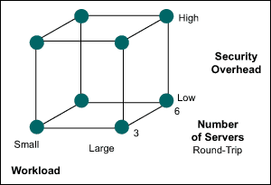
Figure 1: Full Factorial Design Three Factors and Two Levels

The eight test cases depicted in Figure 1 allow for the isolation of the impacts of each factor on the test results (response time), and for the quantification of interactions (beyond the scope of this article). In a full factorial, a test designer gets all the information, but must pay for it. Three factors at two levels are easy enough to study exhaustively, but more factors and levels require more resources. Six factors, for example, at just two test levels each, call for 64 cases in a full factorial. The information paid for in running such a large test set would include the isolation of the effects of complex interactions (3-,4-,5- and 6-way) that are very rarely important. Experimenters, like testers, strive to focus resources on the information most likely to be valuable, and they see the inefficiency in large factorial designs. Interest in spending less time and effort to uncover the specific behaviors of interest usually favors fractional factorial designs in test settings.

Fractional Factorial Designs

As the name indicates, a fractional factorial looks at a subset of all possible combinations. Not just any subset though. There is a smart way to skip and keep test cases so that the smaller plan has a good chance of learning most of what the larger plan would have. A look at the logic and then a walk through of the uses and risks would valuable.

Looking at Figure 1, a good question is: "If you only had time to run four tests (not eight), which four would you run?" A little thinking will probably result in what DOE suggests – a plan like the one shown in Figure 2.

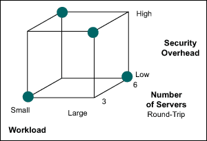
: Figure 2: Fractional Factorial Design

The four test cases depicted in Figure 2, do a pretty good job covering the domain of the complete set of tests. Thinking in the geometry of the illustration, each face of the three-factor cube is covered with two 2 test cases. The test result for each missing case can be estimated using the combined information from the included cases. The logic in such a design is – if the behavior of the system under test is fairly "continuous" – what gets learned in the four test cases that are run can be used to interpolate what would be expected at the cases that were not run.

What does it mean to be continuous? Factors like workload and number of servers probably each influence the overall response time in a smooth, additive way. More or less workload and/or more servers likely push the response time up or down in a reasonably behaved way. There are not big spikes up or down at unknown points. In contrast, if the factors were application and file type (graphics, text), there could well be a certain combination that is quite unlike any others. Trying to study the part in order to know more about the whole could be futile. Unfortunately this cannot be reduced to a simple rule set. However, knowing about the nature of the performance being tested can to guide the tester toward or away from fractional test designs.

Fractional Factorial Case Example

An example helps illustrate the workings and potential limits of a fractional approach. A team decides to test for response time in system with the three factors (workload, number of servers and security overhead), and using just four test cases illustrated on the cube. Each test result for response time (unitless for simplicity) for each factor combination is shown at its corresponding location on the test case cube (Figure 3). Response time is considered a "fail" when above 300.

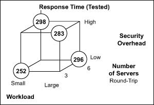
Figure 3: Fractional Test Design Response Time Measured in Four Test Cases

As mentioned, the cases that are included in a fractional design can be used to predict the results for cases not done. None of the tested cases failed, but the results were used to interpolate the untested cases. Figure 4 illustrates those predicted values.

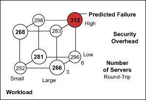
Figure 4: Fractional Test Design Predicted Response Times for Cases Not Run

In this case, the fractional data suggests that the case in the upper right corner of the cube could be a "fail" condition (response time greater than 300). Actual testing at the point bears that out.

Table 2: Predicted Versus Actual Response Times at Points Initially Untested
Test Cases			Response Time
Workload	Servers	Security	Predicted	Actual
Small	3	High	268.04	264.8
Small	6	Low	281.40	260.8
Large	3	Low	266.36	277.7
Large	6	High	312.20	302.8

Looking at Fractional DOE Drawbacks and Risks

The case so far describes a situation where a fractional approach paid off. Testers are not always so lucky. As discussed, if one or more factors influences the test result in a discontinuous way or if there are large unaccounted interactions between the factors, a single point that is left out in a fractional design can be the one place that the system comes to its knees. Where that concern is active there is no substitute for actually observing the cases with highest risk.

It should be noted that there are interim strategies that combine fractional designs supplemented with cases of special risk (and perhaps excluding cases known to be very low risk). Some DOE software offers "D-optimal" designs, which basically ask for information about:

How many cases are there time and resources to do
The factor effects and interactions to study
Any test cases that should be excluded (already tested or impractical)
Any test cases that should be included (special risk or interest)

From there, D-optimal design software searches for the best set of test cases that fit the test needs and resource constraints.

Looking at More Test Factor Combinations

A quick tour of a larger fractional test case may round out the picture a bit. The test setting for the three factors used here actually includes three others as well – Client CPU (2.8, 4.0) Server CPU (3.5, 4.5), and data compression (light, complex). Testing response time for all six factor combinations would call for 64 cases (26).

A fractional design of only eight cases was used, replicating each test (to observe response time variation) to give a total of 16 test cases. This is still just 25 percent of the exhaustive plan.

Figure 5, showing the distribution of results, indicates that about 25 percent of the cases were failures.

Table 3 sorts the results, isolating the failures. It can be seen that no one factor is responsible for the failures. As expected, it is the combined effect of all the factors in concert that drive the overall result. Using that rule of thumb in this case, every factor except Client CPU could be deemed significant. There is a lot more involved in interpreting these outputs, but the focus here is only on the simple basics.

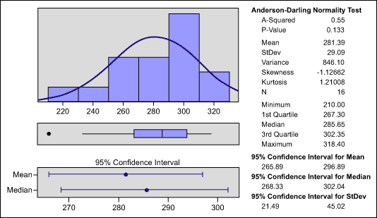
Figure 5: Distribution of Test Results

Table 3: The Sorted Details – Failures Top the List
Workload	Client CPU	Server CPU	Compression	Security	Servers	Response Time
Large	2.8	3.5	Light	Low	6	318.4
Large	4.0	4.5	Complex	High	6	310.7
Small	2.8	3.5	Complex	High	6	308.0
Large	2.8	3.5	Light	Low	6	302.5
Small	4.0	3.5	Light	High	3	301.9
Large	2.8	4.5	Light	High	3	299.6
Small	2.8	3.5	Complex	High	6	298.3
Large	4.0	4.5	Complex	High	6	290.1
Large	2.8	4.5	Light	High	3	281.2
Large	4.0	3.5	Complex	Low	3	275.4
Small	4.0	4.5	Light	Low	6	272.4
Large	4.0	3.5	Complex	Low	3	268.8
Small	4.0	3.5	Light	High	3	266.8
Small	4.0	4.5	Light	Low	6	265.3
Small	2.8	4.5	Complex	Low	3	232.9
Small	2.8	4.5	Complex	Low	3	210.0

Figure 6 shows how the analysis of variance (ANOVA) can be used to single out the impacts of each factor on the test result. The slope of each line provides a quick visual cue to each factor's relative impact. Client CPU has the least impact (almost a flat line) and number of servers has one of the strongest impacts.

ANOVA further quantifies factor effects, as shown in Table 4. The "sequential sum of squares" for each factor gets larger as the factor shows more influence, and the p-value for each factor gets smaller (in its 0-to-1 probability scale) as the factor influence is seen as statistically more significant. Experimenters often use a p-value threshold of about 0,10, view factors with values below that level as worthy of attention and inclusion in the model.

With this plan, the failures detected and those predicted (for the untested cases) found about 95 percent of the fail conditions that were uncovered in a follow-up exhaustive test. There is no guarantee, of course, that any particular application will find similar results.

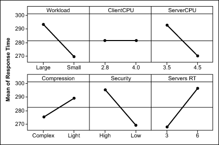
Figure 6: Factor Effects on Response Time

Table 4: Analysis of Variance for Response Time, Using Adjusted Sum of Squares for Tests
Source	DF	Seq.SS	Adj.SS	Adj.MS	F	P
Workload	1	2282.5	2282.5	2282.5	13.17	0.005
Client CPU	1	0.0	0.0	0.0	00.00	0.993
Server CPU	1	1978.0	1978.0	1978.0	11.41	0.008
Compression	1	810.8	810.8	810.8	04.68	0.059
Security	1	2779.9	2779.9	2779.9	16.04	0.003
Servers	1	3280.4	3280.4	3280.4	18.93	0.002
Error	9	1559.8	1559.8	173.3
Total	15	12691.4
S = 13.1646 R-Sq = 87.71% R-Sq (adj) = 79.52%

Conclusion: Another Tool for the Test Kit

Experimenters and testers share the need to develop efficient plans for characterizing the behaviors of systems. Fractional factoral and D-optimal designs offer some options that are useful for testers to understand. If the nature of a system being tested suggests that "spot learning' at fractional design points will provide useful coverage of the whole, then such a plan can be a time-saver. The prospect of savings, though, comes with a big responsibility to know what's being left out in fractional cases. Never expect to get something for nothing – the cases not included in a fractional design carry risk that the test designer must understand. All that said, this is another tool for the test kit.